Plotting formation tops

It would be nice to add formation tops to a plot. Even better, if we already have the data, it would be nice not to have to manually enter them. Let’s walk through an example. Here’s a file from Kansas Geological Survey.

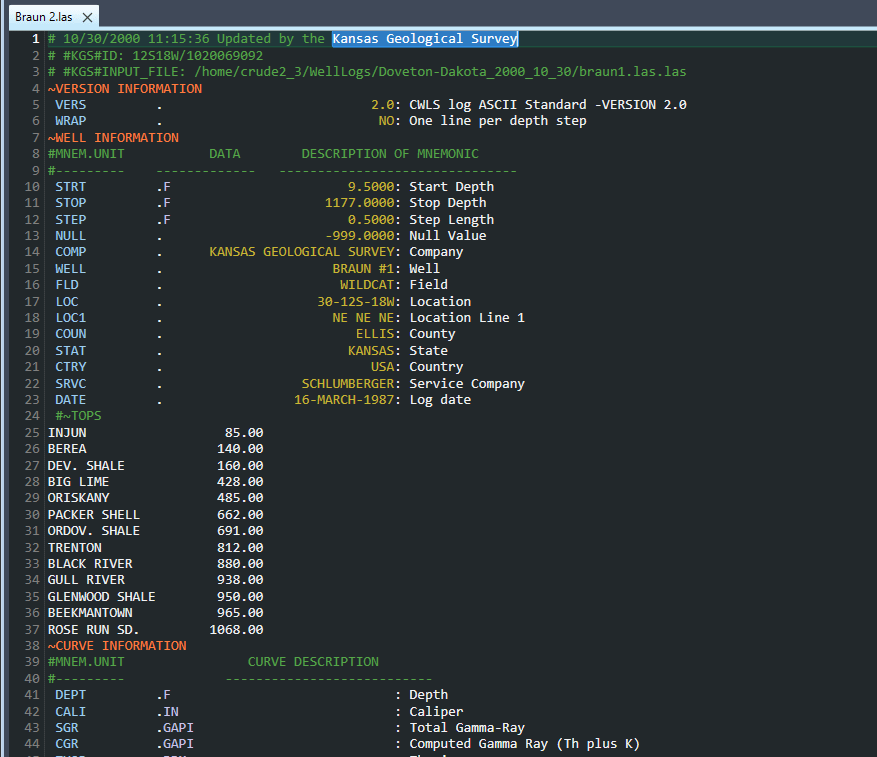
We might have some formation data in another file, but this is a great LAS file to use for our example, because someone put the formation tops right into the file. (A passing note: the lines that represent the tops appear in white, as they are actually not valid lines, according to the LAS 2.0 Standard. They should be commented out, or better yet moved to the ~Other section).

Let’s use the Quick Plots feature (in the Data menu, or else just press Shift + F7). Before we do that, though, let’s copy the lines containing the formation tops (lines 25-37), we’ll need that in a minute.

Nice, Quick Plots gives us one plot for each curve. This is great for seeing what the data in the file looks like. Of course we can configure this differently, this is just the default. For this example, the only change we want to make is to put our formation tops somewhere. You can show these as text annotations with lines, on any track. To make things less noisy, let’s just add a separate, blank track. You can insert a track quickly by right clicking on an existing track, then selecting from the context menu to insert a track before or after the selected one. That brings up the plot configuration dialog, with the new track focused. When we click on the tab below the track configuration titled “Text and lines”, it will look like this:

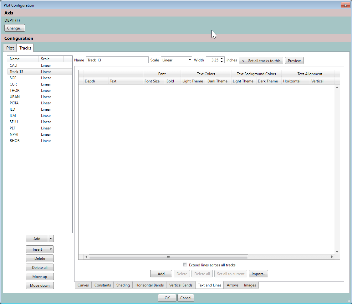
Next we click on the ‘Import’ button to open the Import dialog. Here we can browse to a file, if that’s where the tops are, but we have the rows of text in the clipboard already, and we just paste them in. (Notice the 'GBDS...' button here, more on that below).

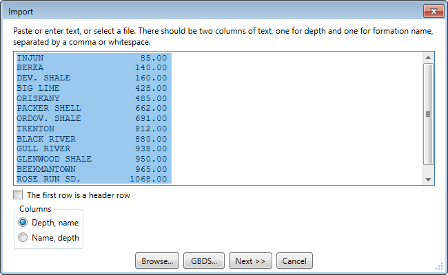
Since the formation tops are in the first column, we need to check the second radio button, "Name, depth". Now let’s click on ‘Next’ and see if that worked.

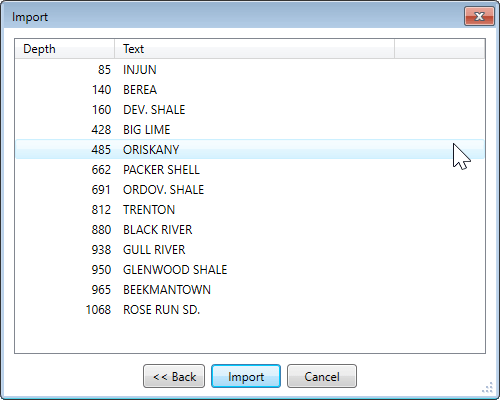
Looks good! Let’s import and see what we have now.

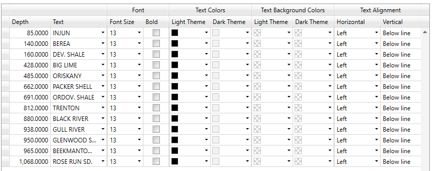
Excellent. Now we could change the font size, line styles and colors. For this example, let’s just do one thing. At the bottom, we’ll check “Extend lines across all tracks”, since all of our tracks are keyed to the same depth scale, and we want to see this information everywhere.

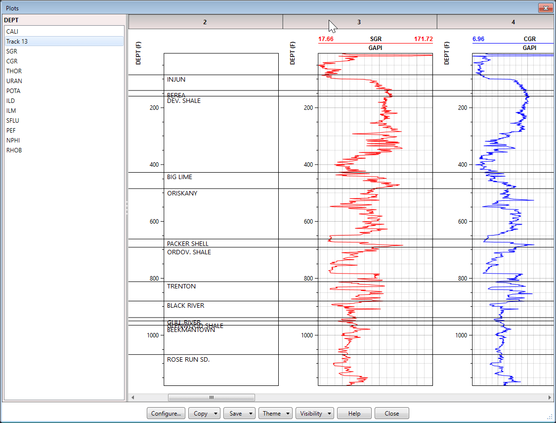
We would probably do a few things at this point to make these look better, such as extending the vertical size of the plots, so the formation top names are not stepping on each other, and it probably would look good to bold the names, maybe make the lines thicker or a different color, etc. But you get the idea. Total time to open the file, create the plots, and insert the formation tops: well less than five minutes!

Do you have the Gulf of Mexico Basin Depositional Synthesis Project (GBDS) database from The University of Texas Institute for Geophysics installed? If so, and you are working with an LAS file from their collection, the program can import formation tops from that database. In this case the 'GBDS' button on the Import dialog will be visible. When you click that, the program will attempt to look up the well in GBDS using the API number. Here is an example of what you might see after a successful lookup.

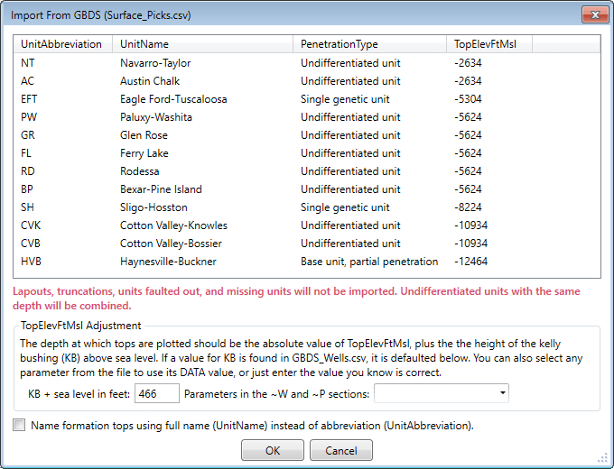
The program will try to locate the KB height value to do the sea level adjustment. If it can't find it, you can select it from the list of parameters available in the file, or else just enter it manually.

Back to blog index